Smoothing a signal

To begin

It has been a while since my last post. I was quite busy at my daily job with a code similarity hashing project. First it was research and development of an algorithm, then productization.

Lately, at already new job, I had a signal processing task. It comprised a couple of stages, smoothing was one of them. This is the kind of problems, which are very simple to imaging and to explain, but their actual solution involves drilling down into minor variants and making tradeoffs. I groked it would be worth a post to describe the solution, at the least for future recollection by my later self.

The problem

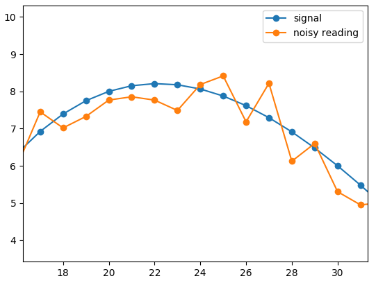
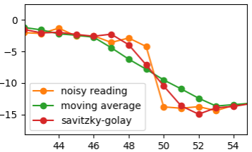
Think of a smooth function. It is being measured every second, but substantial noise alters the original pretty line.

import numpy as np
x = np.linspace(0, 7.5, 76)
y = (x - 1) * (x - 4) * (x - 6)       # The signal
z = y + np.random.random(76) * 2 - 1  # Noisy reading

In development, both the original precise signal and the actual reading were available. This makes the life much easier, since the task definition is straightforward. Measure the difference between the original and the saved signals. Aim to reduce both the maximal difference and the average. In the beginning I involved also the standard deviation, but quickly discovered it isn’t needed, since I was able to bring max and average differences to very low values.

Convolution

Moving average

Many are methods to smooth a signal. It is natural to take a couple of nearby points and “merge” them together under assumption that the noise is random and together those points will eliminate it. Moving average over a window of n = 2 * m + 1 points is: smoothed[i] = sum(z[i - m: i + m + 1]) / n. Meaning, we assume that the original signal is constant at z[i] and we look for a line that is closest to all of points in the [i - m, i + m] range. This takes concise form with:

# https://stackoverflow.com/a/54628145/404099
n = 7
window = np.ones(n) / n
smooth = np.convolve(z, window, mode='same')

In the following form, partial sums are computed in a single run and are expanded by half a window on both sides to allow nearest mode at the edges, with smoothed signal of the same length as the noisy z:

extend = np.ones((n - 1) // 2)  # integer division
z_extended = np.r_[extend * z[0], z, extend * z[-1]]
integral = np.r_[0, np.cumsum(z_extended)]
smooth = (integral[n: ] - integral[: -n]) / n

Savitzky-Golay filter

Of course, real signals are not so constant, as one might wish. Sometimes approximation with higher-level polynomial can yield a better result, be it a straight line, a parabola, a cubic parabola and so on. This is what Savitzky-Golay technique is about. While in moving window every nearby point gets the same weight of 1 / n. It appears that for other degrees, weights can be precomputed in advance. If to consider those weights as another function, the result is kind of “multiplying” one function to another for every index, which is called convolution.

from scipy.signal import savgol_filter)
n = 7          # window length
polyorder = 3  # cubic polinomial approximation
smooth = savgol_filter(z, n, polyorder, mode='nearest')

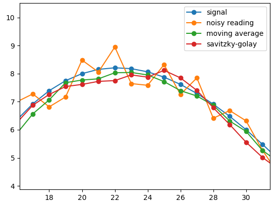
In my task I’ve tried both the simple average and the cubic approximation. I opted to use the former, since the approximation was good enough and it is easy to implement in pure Python and to introduce some customization.

Special cases

1. Edges

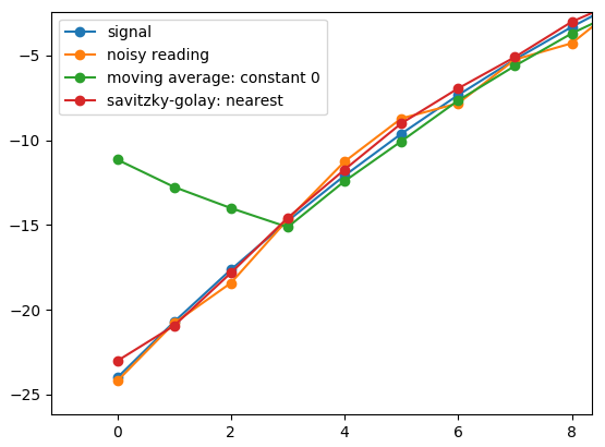
Computing an average of nearby points in the middle doesn’t pose much challenge. Not so easy in the beginning and at the end. In case of the very first point, there are points after, but none before. What to take for z[-1] for the moving window? Many would argue, such points do not matter and can be thrown away. This works good if the signal is long and a few points would not matter. If they do, there are multiple options to choose from depending on the signal nature and your mood. Non-existing points can be set to a constant z[-1] := 0, nearest existing point z[-1] := z[0], mirrored like z[-1] := z[1].

In my case, mirror was the most appropriate choice. Alas it gives less weight to the point itself, while including nearby points twice. So I decided to customize the approach a bit, and reduce window size at the edges to available points only.

2. Very short signal

Well, this possibly only matters to me. But I prefer to work with small and short samples. When there are less data points than the chosen-in-advance window size, every point is “at the edge”. So here, using a constant or a mirror mode would not work nice. Cycle mode would actually yield appropriate results, but it doesn’t apply to the long signal, since in my case it isn’t repeatable. So again adjusting window size worked out nice.

3. Fast level change

Another well known issue with approximation, is that it smooths real changes, unrelated to the noise. Such can be a sudden spike in the data or steep increase or decrease in values that doesn’t get back. Both moving window and Savitzky-Golay approach will reduce the spike, as if caused by the noise and slow down the rapid change. In the middle, finally smoothed signal will get in level with the original. Near the edges, the actual input value will be lost.

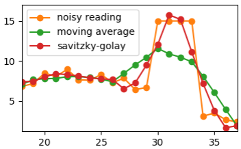
In my specific case, the signal had an additional property, that noise almost vanished in sections of fast change. So smoothing reduced the output quality instead of improving it. Naturally, better simply to detect such sections and discard smoothing there. This can be done, for instance, by noticing a number of points in a raw that are out of standard deviation from the preceding points.