Rotating Rubik's Cube
A short story
My child came to me and showed a nice trick she has discovered with Rubik’s cube. Take one in a solved state. Rotate its right side clockwise, then rotate its down side clockwise. Repeat, and repeat, and repeat. “Daddy, what do you think will happen?” Of course, I knew the answer: it will get back to the solved state. What I didn’t know to tell is how many steps will it take. So we tried to rotate and to count. It get to about one hundred cycles, but we were not sure if every step was counted correctly. This is when I got an idea: what about writing a computer simulation.
I have already tried in the past to introduce programming to the children. Up to now it didn’t work out good enough. This project had a good potential to go better, and it actually have. It serves some real purpose and the task has came from the child herself. It emphasizes what the computers are great at: doing tedious repeating tasks. I have also thought of an easy way to visualize cube state in the process. Beautiful stuff on the screen, which you crafted yourself, is always a pleasure to look at. Finally, the code was of the right size: not too small, and not too big.
Representing the Rubik’s cube
One might have used some 3D rendering for the program to visualize the cube and to allow interactive view from different angles. I opted for simplicity, to remain in the tight bounds of terminal and to write everything in pure Python. For this a flat 2D representation was needed. This is how we did it with print_cube():
  +-+
  |U|
+-+-+-+-+
|L|F|R|B|
+-+-+-+-+
  |D|
  +-+
Here letters stand for the standard names of cube faces: Up, Left, Front, Right, Back, Down. After that we expanded every face into a 3x3 grid, filling cells with letters, that now stand for colors: Blue, Orange, White, Red, Yellow, Green. Our start position looked like this:
         +-+-+-+
         |b|b|b|
         +-+-+-+
         |b|b|b|
         +-+-+-+
         |b|b|b|
         +-+-+-+

+-+-+-+  +-+-+-+  +-+-+-+  +-+-+-+
|o|o|o|  |w|w|w|  |r|r|r|  |y|y|y|
+-+-+-+  +-+-+-+  +-+-+-+  +-+-+-+
|o|o|o|  |w|w|w|  |r|r|r|  |y|y|y|
+-+-+-+  +-+-+-+  +-+-+-+  +-+-+-+
|o|o|o|  |w|w|w|  |r|r|r|  |y|y|y|
+-+-+-+  +-+-+-+  +-+-+-+  +-+-+-+

         +-+-+-+
         |g|g|g|
         +-+-+-+
         |g|g|g|
         +-+-+-+
         |g|g|g|
         +-+-+-+
Output in colors
Well, after seeing the output as above, I told myself: this is indeed a simple terminal way. It is possible to look at the printout and match it with the real cube at hand. All right, but… modern terminals support colors, why not to do a little bit better? The only change needed, was to replace cell content with spaces having color background - start_cube and print it to get:
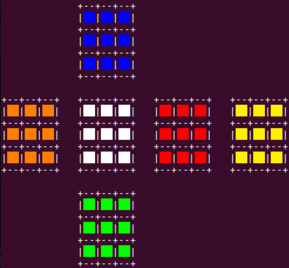
Now a comparison to the real physical cube is much easier. Front side is in White, Blue above is the Up side, and Red - the Right side.

On a technical note, having color prints in terminal is not so difficult. I have made use of ANSI escape codes in the past, even so it usually takes a few attempts to get to the correct code. In this project I was determined to keep things easy and explain everything to my child. This made the choice for colorama to do the job, my first time I’ve used the package.
Rotating side
We have come to modeling side rotation. This is the core part of the project. First, how we rotate a simple planar square? Given a side representation as an array of arrays, this is what rotate_square_clockwise() does. The numbers stand for the first and the second indexes before and after the rotation:
+--+--+--+      +--+--+--+
|00|01|02|      |20|10|00|
+--+--+--+      +--+--+--+
|10|11|12|  ->  |21|11|01|
+--+--+--+      +--+--+--+
|20|21|22|      |22|12|02|
+--+--+--+      +--+--+--+
Complete side rotation involves additional actions. Edges of the adjacent sides should be moved too. Here is how the things move when we rotate_down_clockwise():
                +--+--+--+
                |        |
                +        +
                |   UP   |
                +        +
                |        |
                +--+--+--+

+--+--+--+      +--+--+--+      +--+--+--+      +--+--+--+
|        |      |        |      |        |      |        |
+  LEFT  +      +  FRONT +      + RIGHT  +      +  BACK  +
|        |      |        |      |        |      |        |
+--+--+--+      +--+--+--+      +--+--+--+      +--+--+--+
|20|21|22|  ->  |20|21|22|  ->  |20|21|22|  ->  |20|21|22|
+--+--+--+      +--+--+--+      +--+--+--+      +--+--+--+

                +--+--+--+
                |        |
                + ->     +
                | |DOWN  |
                + ---    +
                |        |
                +--+--+--+
Verification
After implementing the side rotation functions, a simple simulation can run. And - which is crucial for success - we were able to see the result in console and to compare it to the physical cube rotation. The code for the 2 first cycles appears in test_prints().
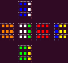
Here goes the first cycle. Begin with the start position. Then rotate right side clockwise:
Now rotate down side clockwise:
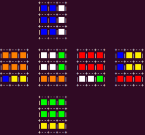
You can notice the problem. Even after two rotations, the colors are not scrambled enough. Rectangles of the same color still appear at every face. Yes, it looks nice to the eye. Alas, this might hide a mistake in the simulation. Of which we had a few by the way. We were able to notice them only after comparison of our simulation output to the rotation of the real cube after 2-3 cycles, when cells get mixed enough. Here’s the output after 2 cycles of right then down sides rotation clockwise:
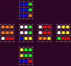
And here is how it appears in reality:

Now the images above match. But the first version of simulation was different. I don’t remember if it took us 2, 3 or 4 cycles to notice that.
Debugging
How to find the error? Again, an easy approach was needed and we thought of such. Use pen and paper, draw a plane representation of the cube with its sides and indexes in each:
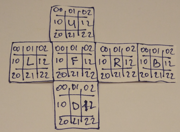
And what is nice about paper 2D models, is that it can be cut and folded into a 3D one:
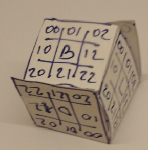
With a folded cube it is much easier to imaging, how pieces are moved during rotation and what cells go where. At this point a few incorrect index switching were spotted and fixed. And finally, our simulation showed the same result as a real cube after 4 test cycles.
Counting the steps
Lastly, to the fun part. I might have described this in some poetic way. Everything is ready, computer is set to do the hard work: run the simulation, crunch the numbers and slowly make progress. Humans fix themselves with a hot drink and just look at the monitor. Indicators tick, steps completed…
Well, it looks good in the movies. And even in day work many optimization and simulation tasks take hours and days. Not in this case. The total number of cycles wasn’t high enough. After several hour long sessions of programming, CPU completed the loop in a few milliseconds. Printouts of cycles blurred on monitor in a blink of an eye, and count_steps() was finished.
Time came to reveal the answer. It is 105. After 105 cycles the cube is returned back to the initial position. Not a trivial number, is it?